8. Differential equations: Part 2

The second lecture on differential equations consists of three parts, each with their own video:

• 8.1. Higher order linear differential equations
• 8.2. Partial differential equations: Separation of variables
• 8.3. Self-adjoint differential operators

Total video length: 1 hour 9 minutes

and at the end of the lecture notes, there is a set of corresponding exercises:

• 8.4. Problems

---

8.1. Higher order linear differential equations

8.1.1 Definitions

In the previous lecture, we focused on first order linear differential equations and systems of such equations. In this lecture, we switch focus to DE's which involve higher derivatives of the function that we would like to solve for. To facilitate this shift, we are going to change notation.

Change of notation

In the previous lecture, we wrote differential equations for $x(t)$. In this lecture we will write DE's of $y(x)$, where $y$ is the unknown function and $x$ is the independent variable. For this purpose, we make the following definitions,

$$y' = \frac{dy}{dx}, \ y'' = \frac{d^2 y}{dx^2}, \ \cdots, \ y^{(n)} = \frac{d^n y}{dx^n}.$$

In the new notation, a linear $n$-th order differential equation with constant coefficients reads

$$y^{(n)} + a_{n-1} y^{(n-1)} + \cdots + a_1 y' + a_0 y = 0.$$

Linear combination of solutions are still solutions

Note that, like it was the case for first order linear DE's, the property of linearity once again means that if $y_{1}(x)$ and $y_{2}(x)$ are both solutions, and $a$ and $b$ are constants,

$$a y_{1}(x) + b y_{2}(x)$$

then a linear combination of the solutions is also a solution.

8.1.2 Mapping to a linear system of first-order DEs

In order to solve a higher order linear DE, we will present a trick that makes it possible to map the problem of solving a single $n$-th order linear DE into a related problem of solving a system of $n$ first order linear DE's.

To begin, define:

$$y_{1} = y, \ y_{2} = y', \ \cdots, \ y_{n} = y^{(n-1)}.$$

Then, the differential equation can be re-written as

$$\begin{split} y_1 ' & = y_2 \\ y_2 ' & = y_3 \\ & \vdots \\ y_{n-1} '& = y_{n} \\ y_{n} ' & = - a_{0} y_{1} - a_{1} y_{2} - \cdots - a_{n-1} y_{n}. \end{split}$$

Notice that these $n$ equations together form a linear first order system, of which the first $n-1$ equations are trivial. Note that this trick can be used to reduce any system of $n$-th order linear DE's to a larger system of first order linear DE's.

Since we already discussed the method of solution for first order linear systems, we will outline the general solution to this system. As before, the general solution will be the linear combination of $n$ linearly independent solutions $f_{i}(x)$, $i \epsilon \{1, \cdots, n \}$, which make up a basis for the solution space. Thus, the general solution has the form

$$y(x) = c_1 f_1 (x) + c_2 f_2 (x) + \cdots + c_n f_{n}(x).$$

Wronskian

To check that the $n$ solutions form a basis, it is sufficient to verify

$$\det \begin{bmatrix} f_1(x) & \cdots & f_{n}(x) \\ f_1 ' (x) & \cdots & f_{n}'(x) \\ \vdots & \vdots & \vdots \\ f^{(n-1)}_{1} (x) & \cdots & f^{(n-1)}_{n} (x) \\ \end{bmatrix} \neq 0.$$

The determinant in the preceding line is called the Wronskian or Wronski determinant.

8.1.3. General solution

To determine particular solutions, we need to find the eigenvalues of

$$A = \begin{bmatrix} 0 & 1 & 0 & \cdots & 0 \\ 0 & 0 & 1 & \cdots & 0 \\ \vdots & \vdots & \vdots & \cdots & \vdots \\ 0 & 0 & 0 & \cdots & 1 \\ -a_0 & -a_1 & -a_2 & \cdots & -a_{n-1} \\ \end{bmatrix}.$$

It is possible to show that

$$\det(A - \lambda I) = -P(\lambda),$$

in which $P(\lambda)$ is the characteristic polynomial of the system matrix $A$,

$$P(\lambda) = \lambda^n + a_{n-1} \lambda^{n-1} + \cdots + a_0.$$

Proof of $\det(A - \lambda I) = -P(\lambda)$

As we demonstrate below, the proof relies on the co-factor expansion technique for calculating a determinant.

$$\begin{align} -\det(A - \lambda I) &= \det \begin{bmatrix} \lambda & -1 & 0 & \cdots & 0 \\ 0 & \lambda & -1 & \cdots & 0 \\ \vdots & \vdots & \vdots & \cdots & \vdots \\ a_0 & a_1 & a_2 & \cdots & a_{n-1} + \lambda \\ \end{bmatrix} \\ &= \lambda \det \begin{bmatrix} \lambda & -1 & 0 & \cdots & 0 \\ 0 & \lambda & -1 & \cdots & 0 \\ \vdots & \vdots & \vdots & \cdots & \vdots \\ a_1 & a_2 & a_3 & \cdots & a_{n-1} + \lambda \\ \end{bmatrix} + (-1)^{n+1}a_0 \det \begin{bmatrix} -1 & 0 & 0 & \cdots & 0 \\ \lambda & -1 & 0 & \cdots & 0 \\ \vdots & \vdots & \vdots & \cdots & \vdots \\ 0 & 0 & \cdots & \lambda & -1 \\ \end{bmatrix} \\ &= \lambda \det \begin{bmatrix} \lambda & -1 & 0 & \cdots & 0 \\ 0 & \lambda & -1 & \cdots & 0 \\ \vdots & \vdots & \vdots & \cdots & \vdots \\ a_1 & a_2 & a_3 & \cdots & a_{n-1} + \lambda \\ \end{bmatrix} + (-1)^{n+1} a_0 (-1)^{n-1} \\ &= \lambda \det \begin{bmatrix} \lambda & -1 & 0 & \cdots & 0 \\ 0 & \lambda & -1 & \cdots & 0 \\ \vdots & \vdots & \vdots & \cdots & \vdots \\ a_1 & a_2 & a_3 & \cdots & a_{n-1} + \lambda \\ \end{bmatrix} + a_0 \\ &= \lambda (\lambda (\lambda \cdots + a_2) + a_1) + a_0 \\ &= P(\lambda). \end{align}$$

In the second last line of the proof, we indicated that the method of co-factor expansion demonstrated above is repeated an additional $n-2$ times. This completes the proof.

With the characteristic polynomial, it is possible to write the differential equation as

$$P(\frac{d}{dx})y(x) = 0.$$

To determine solutions, we need to find $\lambda_i$ such that $P(\lambda_i) = 0$. By the fundamental theorem of algebra, we know that $P(\lambda)$ can be written as

$$P(\lambda) = \overset{l}{\underset{k=1}{\prod}} (\lambda - \lambda_k)^{m_k}.$$

In the previous equation $\lambda_k$ are the k roots of the equations, and $m_k$ is the multiplicity of each root. Note that the multiplicities satisfy $\overset{l}{\underset{k=1}{\Sigma}} m_k = n$.

If the multiplicity of each eigenvalue is one, then solutions which form the basis are then given as:

$$f_{n}(x) = e^{\lambda_1 x}, \ e^{\lambda_2 x}, \ \cdots, \ e^{\lambda_n x}.$$

If there are eigenvalues with multiplicity greater than one, the the solutions which form the basis are given as

$$f_{n}(x) = e^{\lambda_1 x}, \ x e^{\lambda_1 x} , \ \cdots, \ x^{m_{1}-1} e^{\lambda_1 x}, \ etc.$$

Proof that basis solutions to $P(\frac{d}{dx})y(x) = 0$ are given by $f_{k}(x) = x^{m_{k}-1} e^{\lambda_k x}$

In order to prove that basis solutions to the differential equation rewritten using the characteristic polynomial into the form $$P(\frac{d}{dx})y(x) = 0$$ are given by a general formula, taking into account the multiplicity of each eigenvalue: $$f_{k}(x) = x^{m_{k}-1} e^{\lambda_k x}$$ let us first recollect some definitions:

1. A linear $n$-th order differential equation with constant coefficients reads $$y^{(n)} + a_{n-1} y^{(n-1)} + \cdots + a_1 y' + a_0 y = 0.$$

2. The general solution will be a linear combination of $n$ linearly independent solutions $f_{i}(x)$, $i \epsilon \{1, \cdots, n \}$, which make up a basis for the solution space. Thus, the general solution has the form: $$y(x) = c_1 f_1 (x) + c_2 f_2 (x) + \cdots + c_n f_{n}(x).$$

3. The key to finding the suitable basis is to rewrite the DEG in terms of its basis solutions using the properties of the characteristic polynomial and the differential operator as its variable: $$P(\frac{d}{dx})f_{k}(x) = 0$$ and thus, in the general form using the fundamental theorem of algebra: $$P(\frac{d}{dx}) f_{k}(x) = \Biggl( \overset{l}{\underset{k=1}{\prod}} \left(\frac{d}{dx} - \lambda_k \right)^{m_k} \Biggr) f_{k}(x) = 0 \, .$$

4. The solutions to this equation are given as: $$f_{k}(x) = e^{\lambda_1 x}, \ e^{\lambda_2 x}, \ \cdots, \ e^{\lambda_n x} \qquad (1 \leq k \leq l \leq n)$$ and for each eigenvalue $\lambda_{k}$ with multiplicity greater than one, $m>1$, there is a subset of size $m$ with solutions corresponding to that eigenvalue; $$f_{k,m_{k}}(x) = e^{\lambda_k x}, \ x e^{\lambda_k x} , \ \cdots, \ x^{m_{k}-1} e^{\lambda_k x}.$$ These solve the differential equation above in the general form: $$P(\frac{d}{dx}) x^{m_{k}-1} e^{\lambda_k x} = \Biggl( \overset{l}{\underset{k=1}{\prod}} \left(\frac{d}{dx} - \lambda_k \right)^{m_k} \Biggr) x^{m_{k}-1} e^{\lambda_k x} = 0 \, .$$

5. The solutions given above can form the basis if their Wronskian is non-zero on an interval (it may vanish at isolated points); $$\det \begin{bmatrix} f_1(x) & \cdots & f_{n}(x) \\ f_1 ' (x) & \cdots & f_{n}'(x) \\ \vdots & \vdots & \vdots \\ f^{(n-1)}_{1} (x) & \cdots & f^{(n-1)}_{n} (x) \\ \end{bmatrix} \neq 0 \, ,$$ and correspondingly, if any eigenvalue has a multiplicity higher than one: $$\det \begin{bmatrix} f_1(x) & \cdots & f_{k}(x) &x f_{k}(x) & \cdots & x^{m_{k}-1} f_{k}(x)& \cdots & f_{l}(x) \\ f_1 ' (x) & \cdots & f_{k}(x)' &[x f_{k}(x)]' & \cdots & [x^{m_{k}-1} f_{k}(x)]' & \cdots & f_{l}'(x) \\ \vdots & \vdots & \vdots & \vdots & \vdots & \vdots & \vdots & \vdots \\ f^{(n-1)}_{1} (x) & \cdots & f^{(n-1)}_{k}(x) &[x f_{k}(x)]^{(n-1)} & \cdots & [x^{m_{k}-1} f_{k}(x)]^{(n-1)}& \cdots & f^{(n-1)}_{l} (x) \\ \end{bmatrix} \neq 0 \, .$$ Computation of the Wronskian can quickly become a tedious task in general. In this case, we can easily observe that the basis functions are linearly independent, because is not possible to obtain any of the solutions from a linear combination of the others!

   For example, $x e^{\lambda_{1}x}$ cannot be obtained from $x^2 e^{\lambda_{1}x}, \, e^{\lambda_{1}x}, \, x e^{\lambda_{2}x}, \cdots \, .$

Example: Second order homogeneous linear DE with constant coefficients

Consider the equation

$$y'' + Ey = 0.$$

The characteristic polynomial of this equation is

$$P(\lambda) = \lambda^2 + E.$$

There are three cases for the possible solutions, depending upon the value of E.

Case 1: $E>0$ For ease of notation, define $E=k^2$ for some constant $k$. The characteristic polynomial can then be factored as

$$P(\lambda) = (\lambda+ i k)(\lambda - i k).$$

Following our formulation for the solution, the two basis functions for the solution space are

$$f_1(x) = e^{i k x}, \ f_2=e^{- i k x}.$$

Alternatively, the trigonometric functions can serve as basis functions, since they are linear combinations of $f_1$ and $f_2$ which remain linearly independent,

$$\tilde{f_1}(x)=\cos(kx), \tilde{f_2}(x)=\sin(kx).$$

Case 2: $E<0$ This time, define $E=-k^2$, for constant $k$. The characteristic polynomial can then be factored as

$$P(\lambda) = (\lambda+ k)(\lambda - k).$$

The two basis functions for this solution are then

$$f_1(x)=e^{k x}, \ f_2(x) = e^{-k x}.$$

Case 3: $E=0$ In this case, there is a repeated eigenvalue (equal to $0$), since the characteristic polynomial reads

$$P(\lambda) = (\lambda-0)^2.$$

Hence, the basis functions for the solution space read

$$f_1(x)=e^{0 x} = 1, \ f_{2}(x) = x e^{0 x} = x.$$

8.2. Partial differential equations: Separation of variables

8.2.1. Definitions and examples

A partial differential equation (PDE) is an equation involving a function of two or more independent variables and derivatives of said function. These equations are classified similarly to ordinary differential equations (the subject of our earlier study). For example, they are called linear if no terms such as

$$\frac{\partial y(x,t)}{\partial x} \cdot \frac{d y(x,t)}{\partial t} \ or$$ $$\frac{\partial^2 y(x,t)}{\partial x^2} y(x,t)$$

occur. A PDE can be classified as $n$-th order according to the highest derivative order of either variable occurring in the equation. For example, the equation

$$\frac{\partial^3 f(x,y)}{\partial x^3} + \frac{\partial f(x,t)}{\partial t} = 5$$

is a $3^{rd}$ order equation because of the third derivative with respect to x in the equation.

To begin with a context, we demonstrate that PDEs are of fundamental importance in physics, especially in quantum physics. In particular, the Schrödinger equation, which is of central importance in quantum physics, is a partial differential equation with respect to time and space. This equation is essential because it describes the evolution in time and space of the entire description of a quantum system $\psi(x,t)$, which is known as the wave function.

For a free particle in one dimension, the Schrödinger equation is

$$i \hbar \frac{\partial \psi(x,t)}{\partial t} = - \frac{\hbar^2}{2m} \frac{\partial^2 \psi(x,t)}{\partial x^2}.$$

When we studied ODEs, an initial condition was necessary in order to fully specify a solution. Similarly, in the study of PDEs an initial condition is required but now also boundary conditions are required. Going back to the intuitive discussion from the lecture on ODEs, each of these conditions is necessary in order to specify an integration constant that occurs in solving the equation. In partial differential equations at least one such constant will arise from the time derivative and likewise at least one from the spatial derivative.

For the Schrödinger equation, we could supply the initial conditions $$\psi(x,0)=\psi_0(x)$$ together with the boundary conditions $$\psi(0,t) = \psi(L, t) = 0$$

This particular set of boundary conditions corresponds to a particle in a box, a situation which is used as the base model for many derivations in quantum physics.

Another example of a partial differential equation common in physics is the Laplace equation

$$\frac{\partial^2 \phi(x,y)}{\partial x^2}+\frac{\partial^2 \phi(x,y)}{\partial y^2}=0.$$

In quantum physics, Laplace's equation is important for the study of the hydrogen atom. In three dimensions and using spherical coordinates, the solutions to Laplace's equation are special functions called spherical harmonics. In the context of the hydrogen atom, these functions describe the wave function of the system and a unique spherical harmonic function corresponds to each distinct set of quantum numbers.

In the study of PDEs, there are no comprehensive overall treatment methods to the same extent as there is for ODEs. There are several techniques which can be applied to solving these equations and the choice of technique must be tailored to the equation at hand. Hence, we focus on some specific examples that are common in physics.

8.2.2. Separation of variables

Let us focus on the one-dimensional Schrödinger equation of a free particle:

$$i \hbar \frac{\partial \psi(x,t)}{\partial t} = - \frac{\hbar^2}{2m} \frac{\partial^2 \psi(x,t)}{\partial x^2}.$$

To attempt a solution, we will make a separation ansatz,

$$\psi(x,t)=\phi(x) f(t).$$

Separation ansatz

The separation ansatz is a restrictive ansatz, not a fully general one. In general, for such a treatment to be valid, an equation and the boundary conditions given with it have to fulfill certain properties. In this course however, you will only be asked to use this technique when it is suitable.

General procedure for the separation of variables:

1. Substituting the separation ansatz into the PDE,

   $$i \hbar \frac{\partial \phi(x)f(t)}{\partial t} = - \frac{\hbar^2}{2m} \frac{\partial^2 \phi(x)f(t)}{\partial x^2}$$ $$i \hbar \dot{f}(t) \phi(x) = - \frac{\hbar^2}{2m} \phi''(x)f(t).$$

   Notice that in the above equation the derivatives on $f$ and $\phi$ can each be written as ordinary derivatives, $\dot{f}=\frac{df(t)}{dt}$, $\phi''(x)=\frac{d^2 \phi}{dx^2}$. This is so because each one is a function of only one variable.

2. Next, divide both sides of the equation by $\psi(x,t)=\phi(x) f(t)$,

   $$i \hbar \frac{\dot{f}(t)}{f(t)} = - \frac{\hbar^2}{2m} \frac{\phi''(x)}{\phi(x)} = constant := \lambda.$$

   In the previous line we concluded that each part of the equation must be equal to a constant, which we defined as $\lambda$. This follows because the left hand side of the equation only has a dependence on the spatial coordinate $x$, whereas the right hand side only has dependence on the time coordinate $t$. If we have two functions $a(x)$ and $b(t)$ such that $a(x)=b(t) \quad \forall x, \quad t \in \mathbb{R}$, then $a(x)=b(t)=const$.

3. The constant we defined, $\lambda$, is called a separation constant. With it, we can break the spatial and time dependent parts of the equation into two separate equations,

   $$i \hbar \dot{f}(t) = \lambda f(t)$$

   $$-\frac{\hbar^2}{2m} \phi''(x) = \lambda \phi(x) .$$

To summarize, this process has broken one partial differential equation into two ordinary differential equations of different variables. In order to do this, we needed to introduce a separation constant, which remains to be determined.

8.2.3. Boundary and eigenvalue problems

Continuing on with the Schrödinger equation example from the previous section, let us focus on the spatial part

$$-\frac{\hbar^2}{2m} \phi''(x) = \lambda \phi(x),$$ $$\phi(0)=\phi(L)=0.$$

This has the form of an eigenvalue equation, in which $\lambda$ is the eigenvalue, $- \frac{\hbar^2}{2m} \frac{d^2}{dx^2}[\cdot]$ is the linear operator and $\phi(x)$ is the eigenfunction.

Notice that this ordinary differential equation is specified along with its boundary conditions. Note that in contrast to an initial value problem, a boundary value problem does not always have a solution. For example, in the figure below, regardless of the initial slope, the curves never reach $0$ when $x=L$.

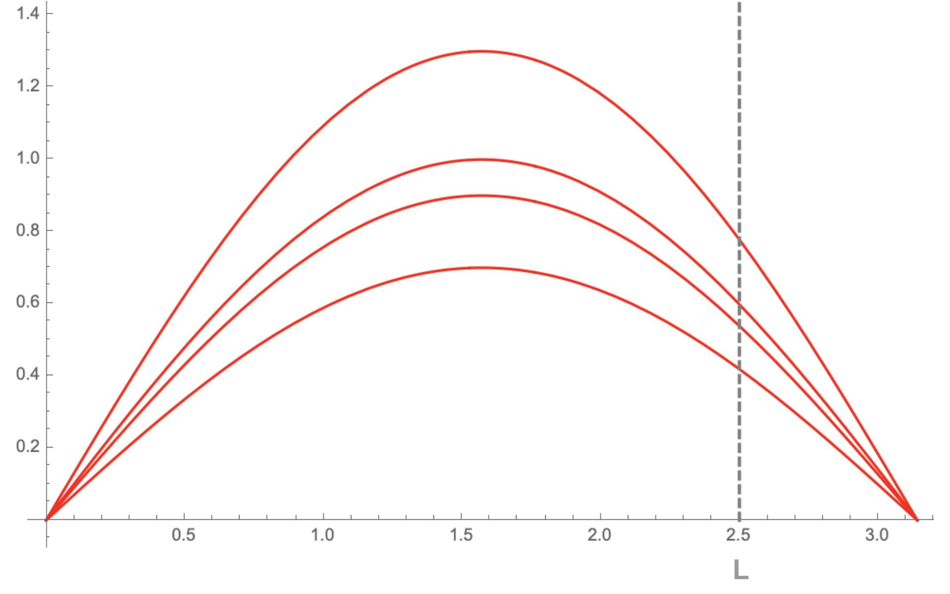
For boundary value problems like this, there are only solutions for particular eigenvalues $\lambda$. Coming back to the example, it turns out that solutions only exist for $\lambda>0$.

This can be shown quickly, feel free to try it!

For simplicity, define $k^2:= \frac{2m \lambda}{\hbar^2}$. The equation then reads

$$\phi''(x)+k^2 \phi(x)=0.$$

Two linearly independent solutions to this equation are

$$\phi_{1}(x)=\sin(k x), \ \phi_{2}(x) = \cos(k x).$$

The solution to this homogeneous equation is then

$$\phi(x)=c_1 \phi_1(x)+c_2 \phi_2(x).$$

The eigenvalue, $\lambda$, as well as one of the constant coefficients, can be determined using the boundary conditions.

$$\begin{align}\phi(0) &=0 \ \Rightarrow \ \phi(x)=c_1 \sin(k x), \ c_2=0. \\ \phi(L) &=0 \ \Rightarrow \ 0=c_1 \sin(k L) \end{align} \, .$$

In turn, using the properties of the $\sin(\cdot)$ function, it is now possible to find the allowed values of $k$ and hence also $\lambda$. The previous equation implies,

$$k L = n \pi, \, n \in \mathbb{N}$$

$$\lambda_n = \big{(}\frac{n \pi \hbar}{L} \big{)}^2.$$

The values $\lambda_n$ are the eigenvalues. Now that we have determined $\lambda$, it enters into the time equation, $i \hbar \dot{f}(t) = \lambda f(t)$ only as a constant. We can therefore simply solve,

$$\dot{f}(t) = -i \frac{\lambda}{\hbar} f(t)$$

$$f(t) = A e^{\frac{-i \lambda t}{\hbar}}.$$

In the previous equation, the coefficient $A$ can be determined if the original PDE is supplied with an initial condition.

Putting the solutions to the two ODEs together and redefining $\tilde{A}=A \cdot c_1$, we arrive at the solutions for the PDE,

$$\psi_n(x,t) = \tilde{A}_n e^{-i \frac{\lambda_n t}{\hbar}} \sin(\frac{n \pi x}{L}).$$

Notice that there is one solution $\psi_{n}(x,t)$ for each natural number $n$. These are also very special solutions that are important in the context of physics. We will next discuss how to obtain the general solution in our example.

8.3. Self-adjoint differential operators

8.3.1. Connection to Hilbert spaces

As hinted earlier, it is possible to re-write the previous equation by defining a linear operator, $L$, acting on the space of functions which satisfy $\phi(0)=\phi(L)=0$:

$$L[\cdot]:= \frac{- \hbar^2}{2m} \frac{d^2}{dx^2}[\cdot].$$

Then, the ODE can be written as

$$L[\phi]=\lambda \phi.$$

This equation looks exactly like, and it turns out to be, an eigenvalue equation!

Connecting function spaces to Hilbert spaces

Recall that a space of functions can be transformed into a Hilbert space by equipping it with a inner product,

$$\langle f, g \rangle = \int^{L}_{0} dx f^*(x) g(x)$$

Use of this inner product also has utility in demonstrating that particular operators are Hermitian. The term "Hermitian" is precisely defined below. Of considerable interest is that Hermitian operators have a set of convenient properties including all real eigenvalues and orthonormal eigenfunctions.

The nicest type of operators for many practical purposes are Hermitian operators. In quantum physics, for example, all physical operators must be Hermitian.

Hermiticity of an operator

Denote a Hilbert space $\mathcal{H}$. An operator $H: \mathcal{H} \mapsto \mathcal{H}$ is said to be Hermitian if it satisfies $$\langle f, H g \rangle = \langle H f, g \rangle \ \forall \ f, \ g \ \epsilon \ \mathcal{H}.$$

Now, we would like to investigate whether the operator we have been working with, $L$, satisfies the criterion of being Hermitian over the function space $\phi(0)=\phi(L)=0$ equipped with the inner product defined above (i.e. it is a Hilbert space).

1. First, denote this Hilbert space $\mathcal{H}_{0}$ and consider $f, \ g \ \in \ \mathcal{H}_0$ which are two functions from the Hilbert space. Then, we can investigate $$\langle f, L g \rangle = \frac{- \hbar^2}{2m} \int^{L}_{0} dx f^*(x) \frac{d^2}{dx^2}g(x).$$

2. In the next step, use the fact that it is possible to do integration by parts in the integral, $$\langle f, L g \rangle = \frac{+ \hbar^2}{2m} ( \int^{L}_{0} dx \frac{d f^*}{dx} \frac{d g}{dx} - [f^*(x)\frac{d g}{dx}] \big{|}^{L}_{0} )$$ The boundary term vanishes due to the boundary conditions $f(0)=f(L)=0$, which directly imply $f^*(0)=f^*(L)=0$.

3. Now, integrate by parts a second time $$\langle f, L g \rangle = \frac{- \hbar^2}{2m} (\int^{L}_{0} dx \frac{d^2 f^*}{dx^2} g(x) - [\frac{d f^*}{dx} g(x)] \big{|}^{L}_{0} ).$$ As before, the boundary term vanishes, due to the boundary conditions $g(0)=g(L)=0$. After canceling the boundary term, the expression on the right hand side contained in the integral simplifies to $\langle L f, g \rangle$.
4. Therefore, $$\langle f, L g \rangle=\langle L f, g \rangle.$$

Thus, we demonstrated that $L$ is a Hermitian operator on the space $\mathcal{H}_0$. As a hermitian operator, $L$ has the property that its eigenfunctions form an orthonormal basis for the space $\mathcal{H}_0$. Hence, it is possible to expand any function $f \in \mathcal{H}_0$ in terms of the eigenfunctions of $L$.

Connection to quantum states

Recall that a quantum state $|\phi\rangle$ can be written in an orthonormal basis $\{ |u_n\rangle \}$ as $$|\phi\rangle = \underset{n}{\Sigma} \langle u_n | \phi \rangle\, |u_n\rangle.$$

In the case of Hermitian operators, their eigenfunctions play the role of the orthonormal basis. In the context of our running example, the 1D Schrödinger equation of a free particle, the eigenfunctions $\sin(\frac{n \pi x}{L})$ play the role of the basis functions $|u_n\rangle$.

To close our running example, consider the initial condition $\psi(x,0) = \psi_{0}(x)$. Since the eigenfunctions $\sin(\frac{n \pi x}{L})$ form a basis, we can now write the general solution to the problem as

$$\psi(x,t) = \overset{\infty}{\underset{n}{\Sigma}} c_n e^{-i \frac{\lambda_n t}{\hbar}} \sin(\frac{n \pi x}{L}),$$

where in the above we have defined the coefficients as a Fourier coefficient,

$$c_n:= \int^{L}_{0} dx \sin(\frac{n \pi x}{L}) \psi_{0}(x).$$

8.3.2. General recipe for separable PDEs

General recipe for separable PDEs

1. Make the separation ansatz to obtain separate ordinary differential equations.
2. Choose which equation to treat as the eigenvalue equation. This will depend upon the boundary conditions. Additionally, verify that the linear differential operator $L$ in the eigenvalue equation is Hermitian.
3. Solve the eigenvalue equation. Substitute the eigenvalues into the other equations and solve those too.
4. Use the orthonormal basis functions to write down the solution corresponding to the specified initial and boundary conditions.

One natural question is: "What if the operator $L$ from step 2 is not Hermitian?"

• It is possible to try and make it Hermitian by working on a Hilbert space equipped with a different inner product. This means that one can consider modifications to the definition of $\langle \cdot, \cdot \rangle$ such that $L$ is Hermitian with respect to the modified inner product. This type of technique falls under the umbrella of Sturm-Liouville Theory, which forms the foundation for a lot of the analysis that can be done analytically on PDEs.

Another question is of course: "What if the equation is not separable?"

• One possible approach is to try working in a different coordinate system. There are a few more analytic techniques available. However, in many situations, it becomes necessary to work with numerical methods of solution.

---

8.4. Problems

1. [] Which of the following equations for $y(x)$ is linear?

   1. $y''' - y'' + x \cos(x) y' + y - 1 = 0$

   2. $y''' + 4 x y' - \cos(x) y = 0$

   3. $y'' + y y' = 0$

   4. $y'' + e^x y' - x y = 0$

2. [] Find the general solution to the equation

   $$y'' - 4 y' + 4 y = 0.$$

   Show explicitly by computing the Wronski determinant that the basis for the solution space is actually linearly independent.

3. [] Find the general solution to the equation

   $$y''' - y'' + y' - y = 0.$$

   Then find the solution to the initial conditions $y''(0) =0$, $y'(0)=1$, $y(0)=0$.

4. [] Take the Laplace equation in 2D:

   $$\frac{\partial^2 \phi(x,y)}{\partial x^2} + \frac{\partial^2 \phi(x,y)}{\partial y^2} = 0.$$

   1. Make a separation ansatz $\phi(x,y) = f(x)g(y)$ and write down the resulting ordinary differential equations.

   2. Now assume that the boundary conditions $\phi(0,y) = \phi(L,y) =0$ for all y, i.e. $f(0)=f(L)=0$. Find all solutions $f(x)$ and the corresponding eigenvalues.

   3. Finally, for each eigenvalue, find the general solution $g(y)$ for this eigenvalue. Combine this with all solutions $f(x)$ to write down the general solution (we know from the lecture that the operator $\frac{d^2}{dx^2}$ is Hermitian - you can thus directly assume that the solutions form an orthogonal basis).

5. [] Consider the following partial differential equations, and try to make a separation ansatz $h(x,y)=f(x)g(y)$. What do you observe in each case? (Only attempt the separation, do not solve the problem fully)

   1. $\frac{\partial h(x,y)}{\partial x} + x \frac{\partial h(x,y)}{\partial y} = 0.$

   2. $\frac{\partial h(x,y)}{\partial x} + \frac{\partial h(x,y)}{\partial y} + xy\,h(x,y) = 0$

6. [] We consider the Hilbert space of functions $f(x)$ defined for $x \ \epsilon \ [0,L]$ with $f(0)=f(L)=0$.

   Which of the following operators $\mathcal{L}$ on this space is Hermitian?

   1. $\mathcal{L}_1 f(x) = A(x) \frac{d^2 f}{dx^2}$

   2. $\mathcal{L}_2 f(x) = \frac{d}{dx} \big{(} A(x) \frac{df}{dx} \big{)}$